Embracing Uncertainty with Conformal Prediction

Types of Uncertainty

When talking about uncertainty in the context of data science, it’s important to note the distinction between epistemic and aleatoric uncertainty. Epistemic uncertainty arises from a lack of knowledge and can be reduced by gathering more data, while aleatoric uncertainty is a result from the inherent randomness of the question being asked. When considering the question of selling your second hand bike again, one might get closer to the ideal listing price by considering similar bikes on the market first. However, even with perfect knowledge, random factors such as a buyer’s personal preferences introduce variability that can’t be eliminated.

Instead of disregarding this inherent variability, we can incorporate it in our answers by quantifying the uncertainty. More specifically, instead of providing a concise but possibly misleading answer, a range of most likely values is considered, such as intervals for regression problems or sets of most likely classes for classification.

Benefitting fairness & decision making

Quantifying aleatoric uncertainty helps us acknowledge inherent randomness, benefiting fairness and decision making. For example, when evaluating credit applicants, uncertainty quantification leads to a more nuanced risk assessment. This helps ensure that individuals with higher income variability aren’t unfairly penalized for factors beyond their control. Another example can be found in financial investment decisions, where a single point estimate falls short in helping to understand the risks of a potential investment. By quantifying the inherent uncertainty, an investor can decide whether to invest based on their own risk tolerance.

Conformal prediction — step by step

There are many different approaches to quantifying uncertainty, such as ensemble methods, Bayesian neural networks, Monte Carlo dropout, quantile regression and bootstrapping, to name a few. While many of these techniques are worthy of a spotlight, in this blog we will focus on a flexible framework that is gaining significant momentum both in academics and industry: conformal prediction.

Conformal prediction is a model-agnostic framework that is capable of generating a statistically valid prediction interval or set of classes while making limited assumptions about your data. It only relies on the assumption of exchangeability, meaning the data points are assumed to be drawn from the same distribution and their joint distribution remains the same regardless of their order. Conformal prediction works for both regression (point and already probabilistic predictions) and classification problems.

So how does it work? Two key concepts in conformal prediction are the calibration set and nonconformity scores. Conformal prediction in its most basic form follows these steps:

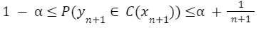
Step 1. The data is split into training and calibration sets. The model is trained as usual, resulting in a predictor for new data points. Since we want a prediction interval with statistical guarantee, the calibration set should be of a certain size. Given the following equation, where a is our specified confidence level, y₍ₙ₊₁₎​ the value/class of the next data point,C(xₙ₊₁) the interval generated for the next input and n the size of the calibration set, we can derive the coverage guarantee.

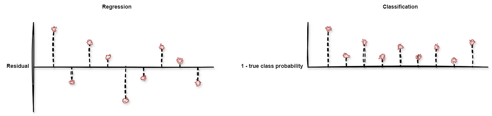
Step 2. For each data point in the calibration set, a nonconformity score is computed. This score can be based on any performance metric, such as a residual error for regressions and class probabilities for classification.

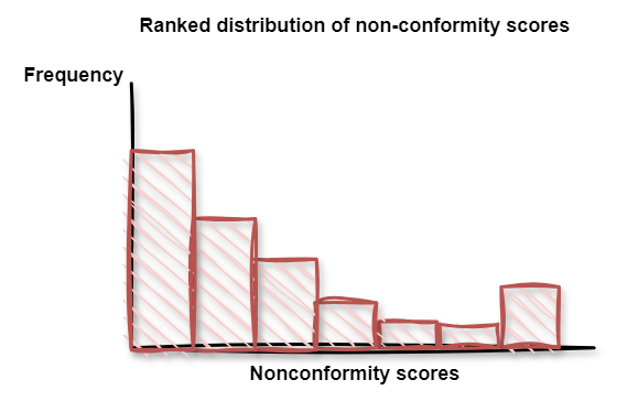
Step 3. The nonconformity scores are ranked to compute a distribution.

Step 4. For this distribution, the specified level of confidence is used to find the relevant threshold.

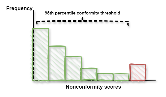
Step 5. For new data points in regression problems, the prediction interval is constructed around the model’s prediction based on the selected quantile from the nonconformity score distribution. 

In a classification context, the selected quantile is used as a threshold for the predicted class probabilities. If multiple classes have a predicted probability higher than the threshold, the model’s output consists of a set of classes.

Step 6. To calibrate or maintain the interval or threshold, the calibration set can be updated over time, making it a robust framework in a nonstationary context.

Conformal prediction in Python

The library crepes allows us to easily implement these steps in Python by providing us with a model wrapper that is compatible with sklearn. Transforming a single point regressor to a model capable of producing a prediction interval would look as follows.

import pandas
from sklearn.ensemble import RandomForestRegressor
from sklearn.model_selection import train_test_split

from crepes import WrapRegressor

# Load data
data = pd.read_csv("used_bikes.csv")
X = data.drop("price", axis=1)
y = data["price"]

# Create a train, calibrate and test set
x_train, x_test, y_train, y_test = train_test_split(X, y, test_size=0.5)
x_train, x_cal, y_train, y_cal = train_test_split(x_train, y_train, test_size=0.25)

# Create a model and calibrate
regressor = WrapRegressor(RandomForestRegressor())
regressor.fit(x_train, y_train)
regressor.calibrate(x_cal, y_cal)

# Produce a prediction interval with specified confidence and minimum values
prediction_interval = regressor.predict_int(x_test, confidence=0.95, y_min=0)

Comparing the generated prediction interval to a single point estimate for the price of second hand bikes:

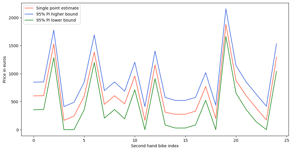
Note that the prediction interval’s width is the same for all bikes. To make the prediction interval more informative, the difficulty of each prediction can be estimated, assigning more difficult data points with a wider interval. One way to normalize the prediction interval is by using the distance to the closest data points, or by considering the standard deviation or absolute error of a prediction relative to its nearest neighbors. Alternatively, when using an ensemble of models, the variance of the predictions of the constituent models can also be used to estimate the difficulty. For more details on the possible normalization methods, please see the documentation here.

All of these options can be done in crepes as well. Since we happen to use a random forest regressor, let’s take a look at the latter approach.

from crepes.extras import DifficultyEstimator

# Estimating the difficulty based on the variance of the underlying models
de_ensemble_var = DifficultyEstimator()
de_ensemble_var.fit(X=X_train, learner=regressor.learner, scaler=True)

rf_norm_var = WrapRegressor(regressor.learner)
rf_norm_var.calibrate(X_cal, y_cal, de=de_ensemble_var)

interval_rf_ensemble = rf_norm_var.predict_int(X_test, confidence=0.95, y_min=0)

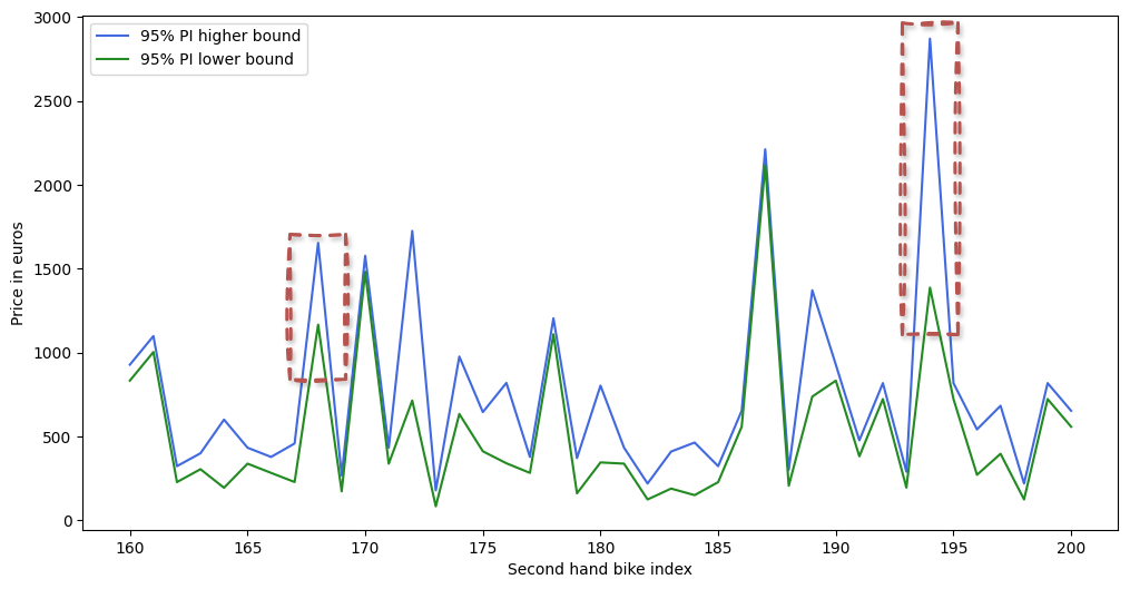
The crepes library allows you to wrap both regression and classification models. Other Python libraries that are interesting to give a look are MAPIE (for use cases such as conformalized quantile regression or time series), TorchCP (specifically for PyTorch) and Venn-ABERS (for classification).

Applications & limitations

These steps and an easy implementation make for a flexible yet robust framework to produce reliable prediction intervals. As a result, the applications of conformal prediction range from ordinal classification at Amazon to reviewing the factual accuracy of LLM output and forecasting in the traffic modeling domain and energy industry.

Although conformal prediction has a lot going for it, it’s important to note some topics for discussion. For instance, the framework does come with an extra computational step to compute nonconformity scores, which might complicate your pipeline when working with larger datasets. On the other side of the spectrum, it can be challenging to use in the context of smaller datasets, since data in the calibration set can not be included in the training set. Finally, in cases where data points are not exchangeable, such as time series data, the prediction intervals require some extra work. An interesting question in applying conformal prediction in the context of time series is that of managing the nonconformity distribution shift over time.

Conclusion

In this blog post, we have made a case for uncertainty quantification through the use of the conformal prediction framework, benefiting both fairness and decision making. If this sparked your interest, please see the following blogs, keynotes and repositories as the next steps into the uncertainty rabbit hole:

• Emmanuel Candes (Stanford University) keynote at NeurIPS on conformal prediction
• Valeriy Manokhins awesome-conformal-prediction repository
• A review of prediction intervals for regression problems
• Calibrating a probabilistic model to accelerate the energy transition