Detecting War Crimes from Space
Building an Open-Source Pipeline with SQLMesh and DuckDB

Tom Uijtdehaag


If you're getting the feeling recently that there's more war in the world, you're right. Compared to 2010 the number of armed conflicts have more than doubled. Centre for Information Resilience (CIR) aims to provide digital witness accounts using open source data and tools. In this blogpost we're going to take a technical deep dive into how we built an open-source pipeline to detect burn events in a collaborative effort between CIR and BigData Republic (BDR).
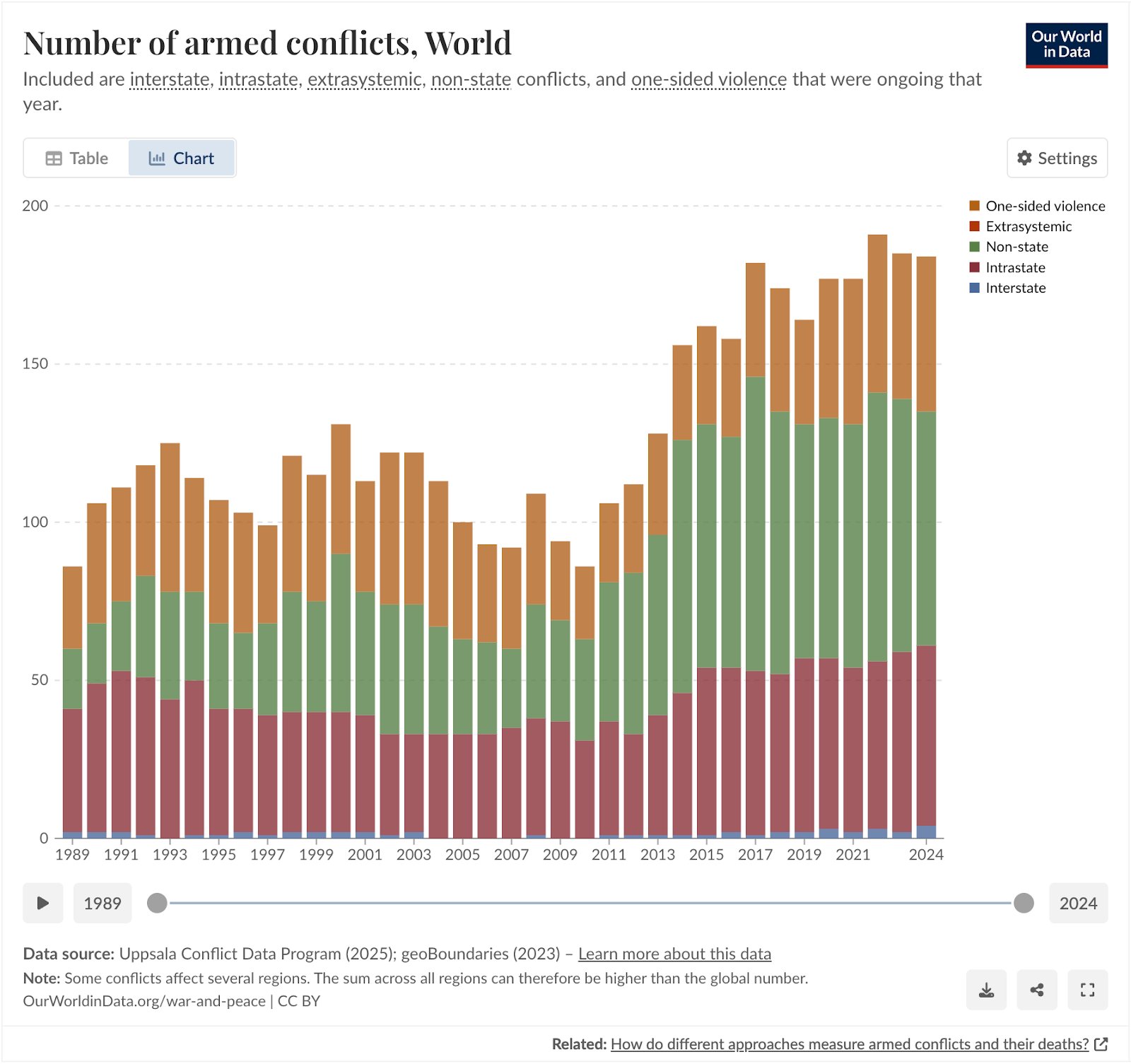
Number of armed conflicts in the world over time. Our World in Data
The conflict in Sudan
The war in Ukraine, and more recently the wars between Israel, Gaza and Iran, have been getting a lot of media attention. Meanwhile, despite claiming more than 150,000 lives and displacing about 12 million people (BBC), global media coverage on the war in Sudan has been sparse. The United Nations has now called the situation in Sudan, that has been escalating since April 2023, the world's largest ongoing humanitarian crisis.
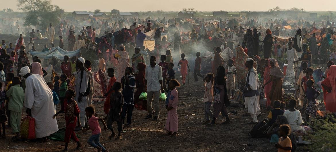
Displaced people arrive in South Sudan from Sudan, through the Joda border crossing. © UNHCR/Ala Kheir
In conflicts like these, atrocities often go unreported, unverified, and unpunished. One such atrocity is the burning of civilian homes. While perpetrators often document themselves while using arson to destroy civilian targets, which is classified as a war crime by the International Criminal Court, documenting and verifying these incidents has proven to be difficult.
CIR's Project Sudan Witness
At CIR, investigators working on the Sudan Witness project are using open-source investigations (OSINV) to change that.
Open-source investigations rely entirely on information that is publicly available, such as satellite imagery, social media posts, news reports, government documents or sensor data. The emphasis is on collecting, verifying and analyzing these open sources to build evidence-based findings, without needing access to classified or insider information.
This approach is widely used by journalists, researchers, and human rights groups to investigate events like conflicts, environmental disasters, or corporate misconduct. Unlike traditional “intelligence,” which suggests secrecy or state use, open-source investigations highlight transparency and verifiability. Anyone can, in principle, retrace the steps and check the evidence.
They have developed a methodology to map the burning of villages remotely using publicly available data sources. I highly recommend reading that if you're interested in learning more about OSINV. It goes into great detail regarding the validation and verification process, including cross-referencing other sources and the spatiotemporal analysis (pinpointing location and time) of those sources.
This methodology is highly relevant to documenting war crimes, as it allows investigators to detect and map burn events with open, verifiable evidence. But there are limits: it can confirm that fires occurred and where, yet it cannot determine intent, identify perpetrators, or establish whether a war crime took place. Instead, these findings serve as supporting evidence that, combined with other verified sources, can help justice and accountability actors build cases.
In this blogpost I will focus on the automation and technical implementation of this methodology, and how we've reduced the time it takes to collect and validate fire detections from hours to minutes. The results have become more consistent and investigators can now spend more time on the actual verification of arson events.
While "we" often refers to CIR and BDR jointly, the methodology and initial automation were developed by CIR. BDR further improved and automated the process for efficiency and consistency. Sections before "Data Engineering: SQLMesh + DuckDB" detail CIR's work; subsequent sections describe BDR's contributions.
Turning OSINV into a System
So let's dive in! Burnt villages often show up in satellite imagery as darkened patches, but finding and verifying them manually is time-consuming. Investigators used to cross-reference NASA fire detections with Sentinel-2 imagery by hand. Now, we’ve built a system that automates large parts, making the process faster, repeatable, and scalable.
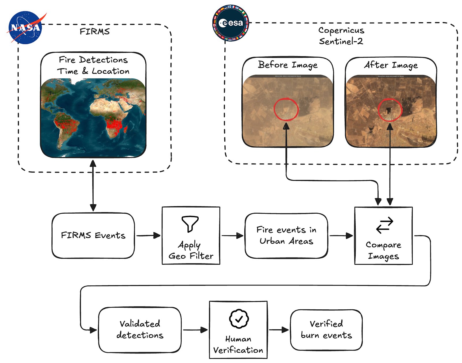
Overview of the Burnscar system. We collect fire detections, filter them and do automated validation before passing them on for human verification.
At a high level the process consists of these four steps:
- Collect fire detections provided by NASA Fire Information for Resource Management System (FIRMS)
- Apply a geospatial filter, so only fires inside urban areas are considered
- Collect and compare before and after imagery from ESA's Sentinel-2 multispectral sensors to detect burn scars
- Verify the remaining detections that are classified to have left burn scars
Note the distinction we make between "Validated" detections and "Verified" burn events here. Throughout this article we use "validation" for the automated processing and classification of satellite imagery, and "verification" for the human verification done by our investigators.
These verified events are finally published on CIR's Map of Fires in Sudan.
Data Sources
To do this, we pull in multiple open datasets:
FIRMS: Fire Detection
NASA’s FIRMS (Fire Information for Resource Management System) delivers near real-time fire detections from satellites. We use it as our starting point. The FIRMS API provides detections per country; these go into our pipeline for validation. The primary components of the detection that we use are coordinates and a timestamp, but FIRMS provides no imagery. Some additional metrics are provided, like brightness of the event and information about the satellite’s instrument that captured the detection, but we're currently not using this.
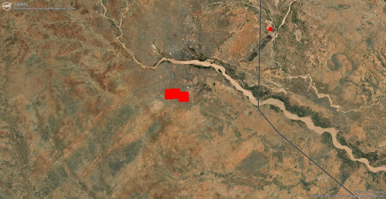
NASA FIRMS Detections as shown on the FIRMS Global Fire Map. These alerts serve as the starting point for our pipeline.
Sentinel-2: Before and After Imagery
Sentinel-2 satellites provide images in visible and infrared bands that allow us to see scarred earth left behind by fires. The near-infrared (NIR / B08) and shortwave infrared (SWIR / B12) bands are especially useful, as burn scars show up clearly here. We fetch before and after imagery via Google Earth Engine (GEE) using the Python SDK.
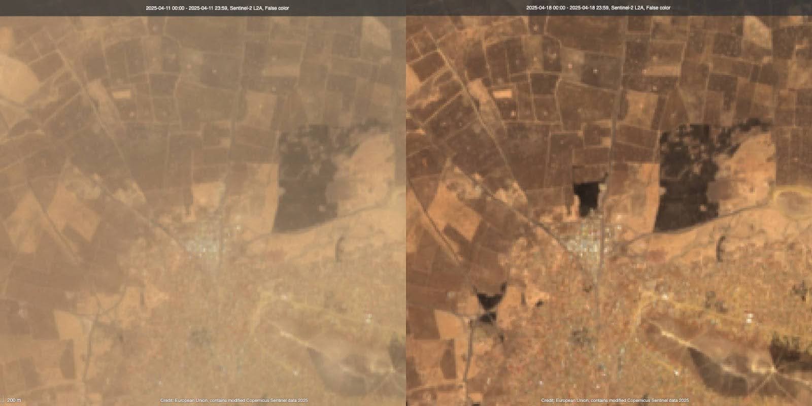
Example of Sentinel-2 Imagery. Some dark patches have appeared in the center and bottom-left quadrant of the image.
Google Research Open Buildings
The Open Buildings dataset by Google Research provides footprints of buildings as geometries. This is useful to assess the potential impact a fire has had on civilian infrastructure. This dataset is accessed through GEE.
GADM: Administrative Boundaries
We use GADM's country and region data to contextualise detections. For instance, tagging a burn event as being in "South Darfur". This adds geographic precision for investigators and is also used to generate contextual links for follow-up searches on platforms like Facebook and X.
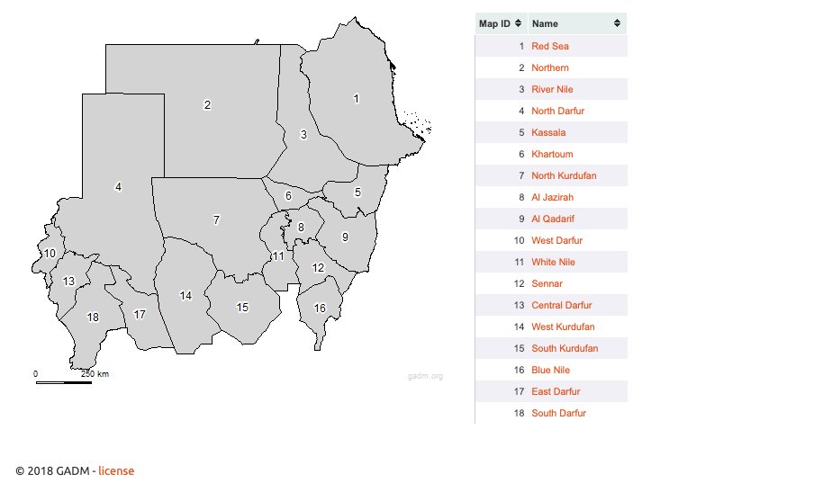
Level 1 regions in Sudan, these are used for cross-validation purposes.
GeoNames: Place Names
Similar to GADM, GeoNames helps us assign names to remote locations. This adds clarity when mapping or reporting events. We also use these names to create pre-filled search links to platforms like X and Facebook, helping analysts discover citizen reporting or social media evidence tied to the location.
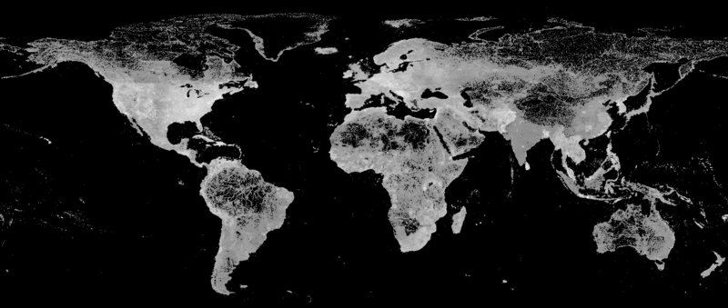
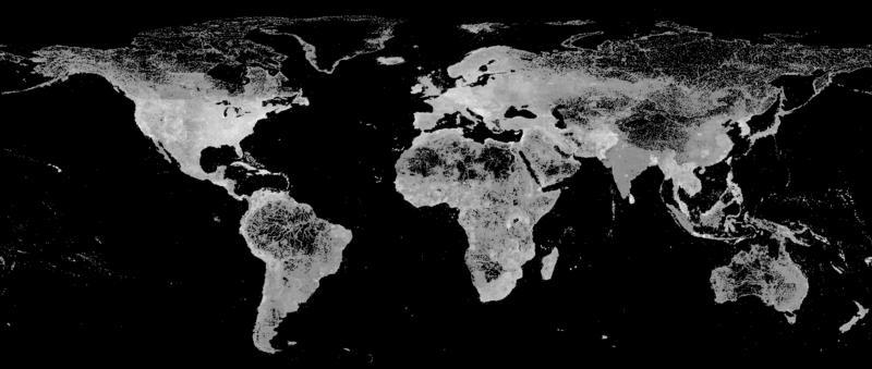
Feature density of the GeoNames database. We use this database to tag burn events with the nearest place names.
Urban Area Filter
We reduce false positives by ignoring detections that occur outside human settlements. We've made a custom geometry for Sudan's urban areas by dissolving Google Open building footprints and buffering them with a fixed radius. This approximation isn’t perfect, but it's a useful filter.
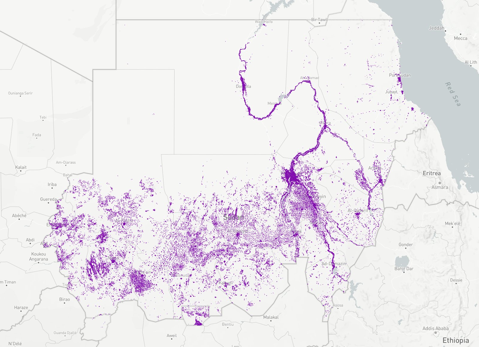
The Urban Areas filter of Sudan. We use this as a geo filter to focus on urban areas only.
The Validation Process
Once a fire detection passes the filters, we kick off a geospatial image analysis workflow in Earth Engine. At a high level this process looks as follows, I'll go through these steps in more detail soon.
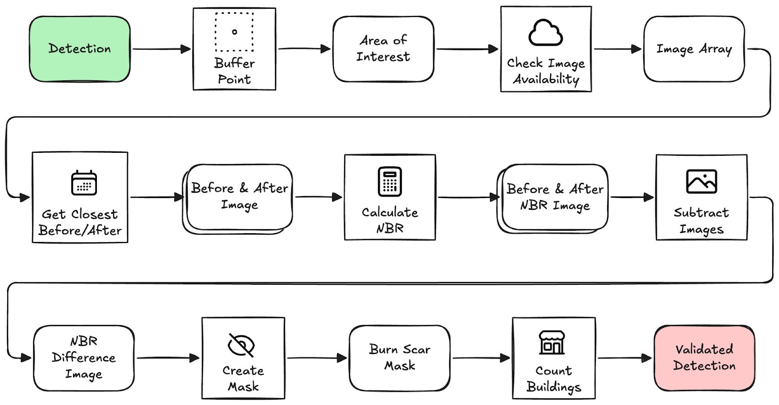
Overview of the validation process. This is the automated process before handing detections off for human verification.
An interesting remark here is that we're just constructing lazily evaluated instructions that will later be sent to the Earth Engine API, so all computation happens remotely and only when some concrete result is requested. For example, creating a FeatureCollection and then applying .filterDate(start_date, end_date) does not make any calls to GEE yet. Only when we access some attribute and call getInfo(), the feature collection is accessed and filtered remotely before returning only the attribute we requested. The code provided here is simplified for the purpose of this blogpost, for the real code please refer to the repository on our GitHub.
1. Buffer the FIRMS detection point to create an area-of-interest (AOI). We use this AOI as bounds for the imagery used in analysis.
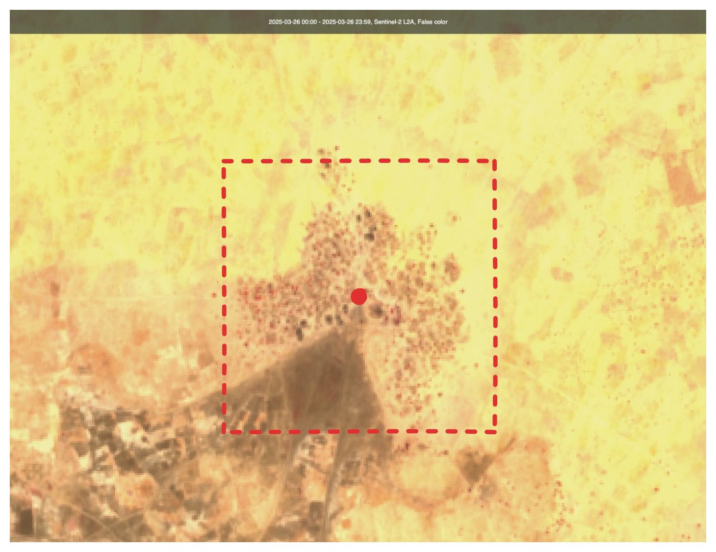
The detection point, with the area of interest visualised. The AOI is used for further steps of the validation process.
2. Check image availability before and after the event, filtering for cloud-free days (less than 10% of pixels are cloudy). Luckily, GEE provides a CLOUDY_PIXEL_PERCENTAGE property that we can filter on.
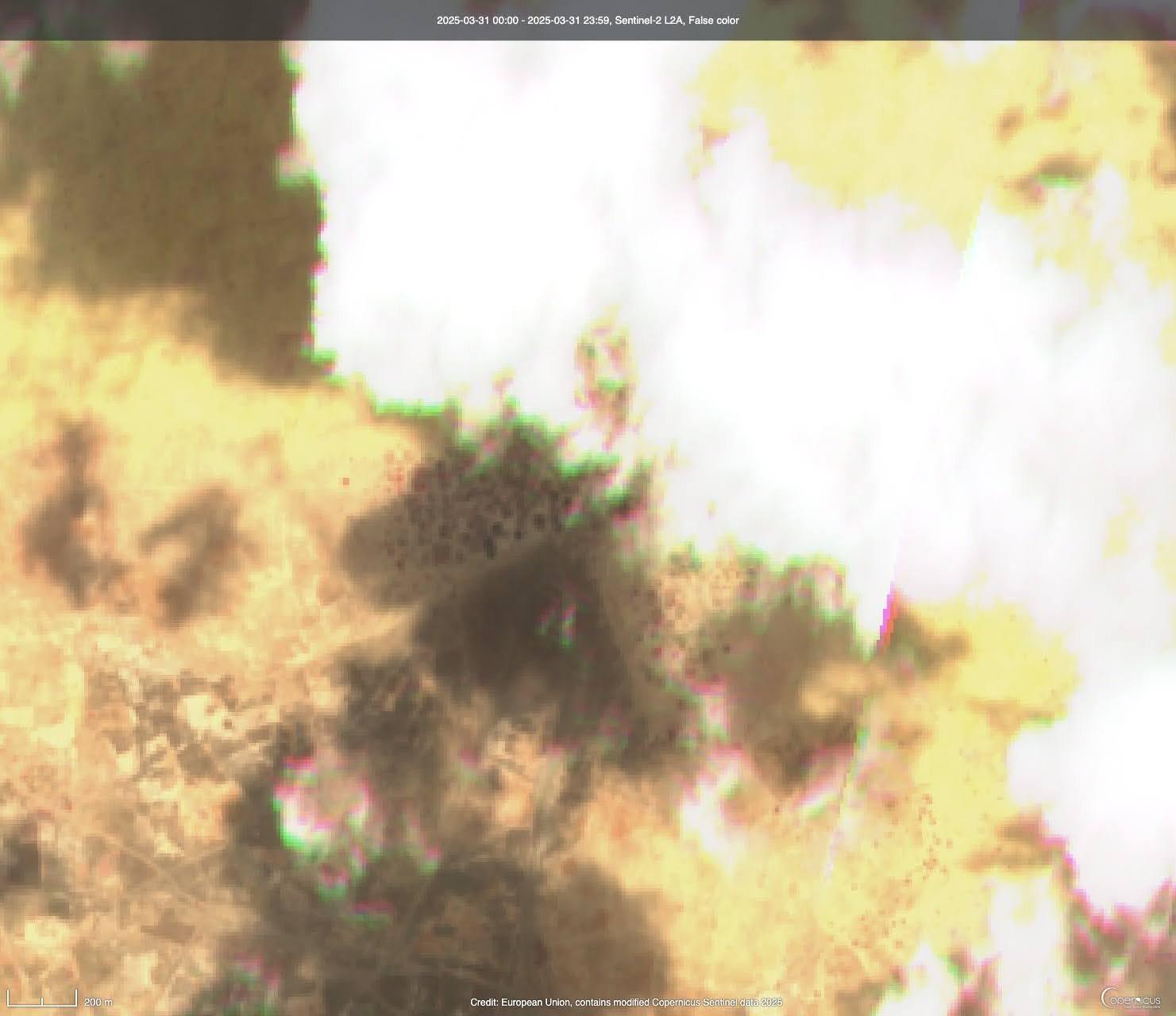
The same location that has cloud cover obstructing our view. Obviously, this image is of little value for our purpose of inspecting burn scars.
3. Fetch closest valid Sentinel-2 images around the event window. We'll use this before and after image for our validation process.
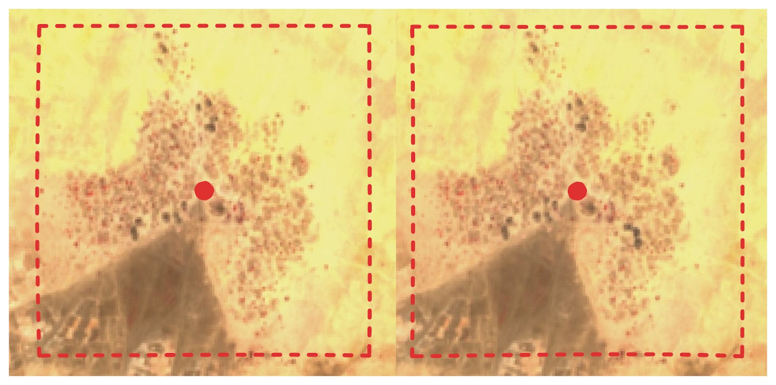
The before and after image, side-by-side. When inspected carefully, we see a dark spot appear in the bottom right quadrant of the after image.
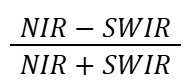
4. Calculate Normalised Burn Ratio for both images to highlight burned areas. The Normalised Burn Ratio (NBR) is an index designed to highlight burnt areas by leveraging reflectance of Near Infrared (NIR) and Shortwave Infrared (SWIR) wavelengths. In the case of Sentinel-2 we're using bands 8 for NIR and 12 for SWIR.
5. Subtract the NBR images to detect the difference in burned surface between the before and after image.
The before and after images, shown here as NIR / SWIR for visibility. Just to the bottom right of the center we see a dark spot appear.
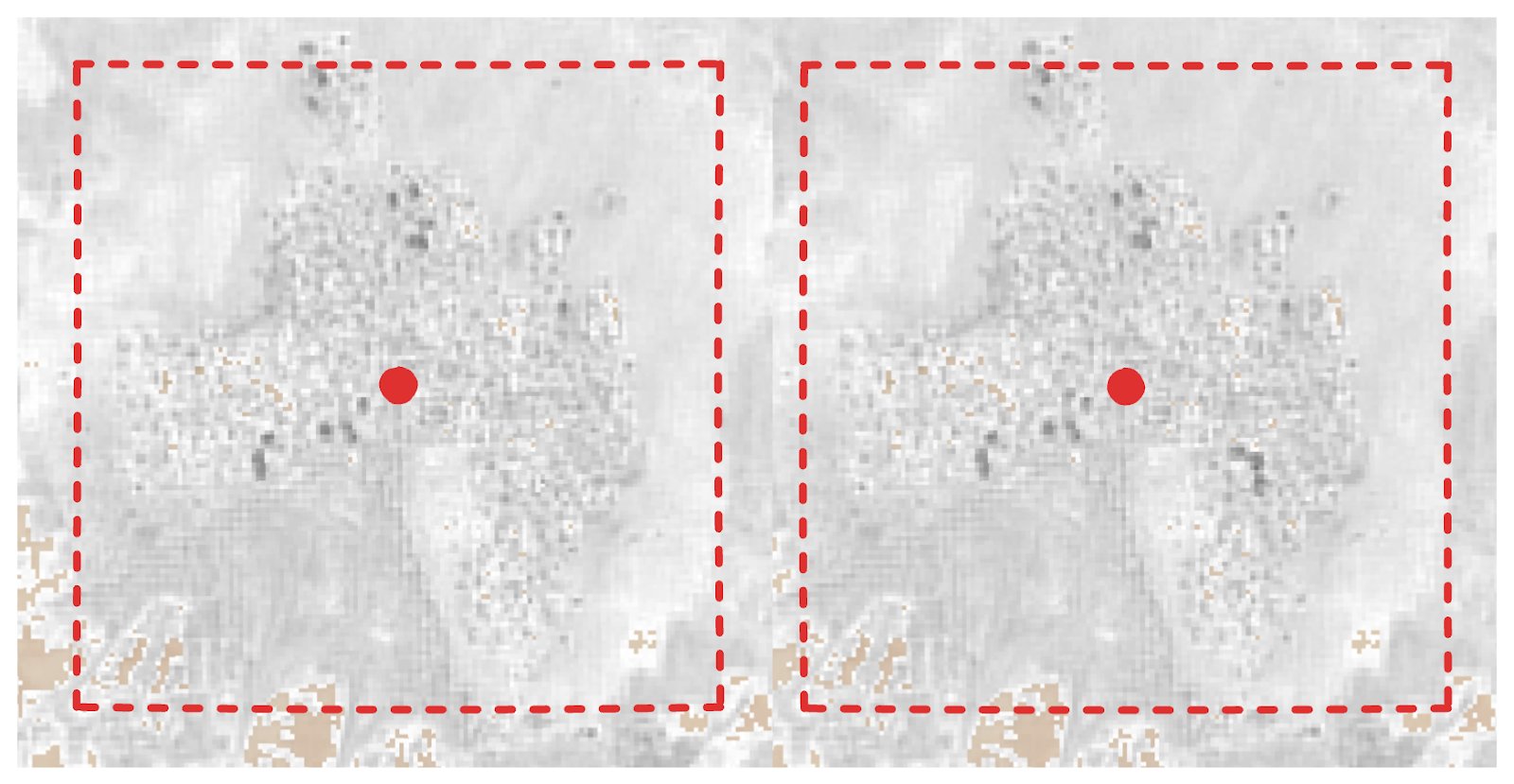
6. Threshold the result to extract likely burn areas, this gives us a binary map that is 1 (white) or 0 (black). Where 1 means this pixel was not burn scarred on the before image, but is on the after image.
The before and after NBR image subtracted from each other (left) and the resulting mask image when we apply a threshold (right). This is basically like cranking up the contrast to 100.
7. Overlay with building footprints and count how many structures are affected. We do this by intersecting the mask with the building's polygons and counting the number of geometries are left.
The building geometries overlaid on the burn scar mask. Just by looking where they overlap, we could say that around 6 buildings have new burn scars on them.
A bunch of information is then compiled into an object. For example before and after dates of the imagery used, burnt pixel count and burnt building count. In case imagery was not available or the available imagery was too cloudy, we set the no_data or too_cloudy flags respectively.
Data Engineering: SQLMesh + DuckDB
A requirement for this project was that it should be able to run locally on an investigators laptop, but at a later stage will be deployed to the cloud. With that in mind we chose to use SQLMesh for organising and orchestrating our data models, and DuckDB as a fast, local, analytical database. Mix in DuckDB's spatial extension and we have a simple but powerful data pipelining system. With some minor adjustments this can (and will) be deployed to run on serverless compute, with the data stored on a cloud object storage.
SQLMesh
SQLMesh manages the pipeline. It's similar to dbt Core, with some very useful additional features. It allows us to write transformations, either as SQL models or as Python models for more complex logic like API interactions. SQLMesh parses schemas from the models and automatically detects dependencies, builds a Directed Acyclic Graph (DAG) and provides column-level lineage out-of-the-box. A model can be defined as incremental by time range, allowing SQLMesh to handle partitioning of our fire detection events. Furthermore, SQLMesh keeps track of the state of our models and is able to efficiently backfill missing data.
*In my opinion.
SQL Models
These handle all the "normal" data transformations. And powered by DuckDB and its Spatial extension, this is the majority of models.
A relatively simple example of a SQL Model in SQLMesh looks like this:
As you can tell, SQLMesh requires some special SQL syntax to define metadata about the model. We specify the kind (which in most cases is FULL, VIEW or INCREMENTAL of some kind), an optional description and audits (in this case we require at least 1 row). The remaining part is just a regular SQL query, which is parsed by SQLMesh using SQLGlot, their open source SQL parser and transpiler.
Python Models
These handle more complex operations that cannot be done with just SQL, like:
- Fetch data from external sources
- Interaction with Earth Engine
- More complex logic for checking and ensuring file presence on disk
For example, our (slightly simplified) model that fetches FIRMS detections from NASA looks like this:
The complexity of the actual API interaction is hidden away in the NASAFetcher, which allows us to write a super simple model and let SQLMesh handle all partitioning and planning using its internal state.
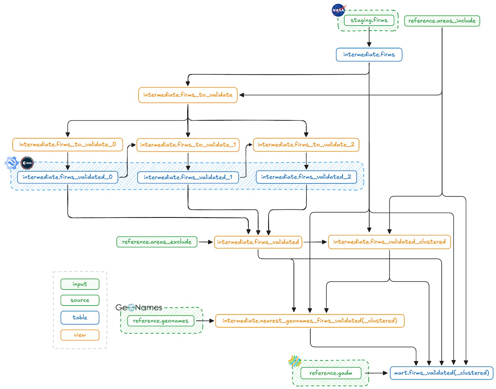
The entire SQLMesh DAG. We'll soon go into more detail on the retry mechanism involving the firms_to_validate_n and firms_validated_n models. The models that end with (_clustered) are actually two variants of a similar model, one for individual detections and one for clustered detections.
DuckDB
We use DuckDB mainly for its processing and analytical capabilities, but it also functions as our storage backend. It simply stores the entire database on disk as a single file. In addition to DuckDB having a lot of built-in functions, modern SQL syntax (like the QUALIFY clause), first-class nested types (which came in very handy as you'll see soon) and reads and writes a range of filetypes from and to disk.
Spatial extension
The spatial extension is what enables geospatial processing in DuckDB. It does so by adding support for the GEOMETRY type and also adds a bunch of geospatial functions. It has allowed us to fully replace GeoPandas from an earlier iteration. Some of the key operations we rely on include:
- Spatial JOINs (ST_Intersects): Returns TRUE if two geometries intersect, or FALSE otherwise. This function allows us to intersect geometries efficiently. For example, filtering FIRMS detections with our Urban Areas filter and adding GADM names to detections.
- Great Circle Distance (ST_Distance_Sphere): Returns minimum distance in meters between two geometries. We use this to add the nearest known GeoName to a detection.
- Within Radius (ST_DWithin): Returns TRUE if the distance of two geometries is within the given limit, or FALSE otherwise. This is used for early filtering in a JOIN condition in combination with ST_Distance_Sphere to limit the number of exact distances we have to calculate.
Centroid Calculation (ST_Centroid): Returns the centroid of a geometry. Used to extract the center point of a cluster of detections. Useful for identifying a single representative location for mapping, reporting, or correlating with external place names like those from GeoNames.
What’s powerful here is that DuckDB handles all this in-memory, with excellent performance, even on large geospatial datasets. And because the pipeline runs locally or inside a lightweight container, we don’t need PostGIS or a dedicated GIS database server, just DuckDB and a flat file.
Challenges Along the Way
The original burnscar implementation sometimes took over an hour to run, involved manual filtering along the way and running a fragmented set of scripts to achieve the final result. We identified a number of improvements to be made, mainly in consistency and speed.
The issues had some different roots:
- Inefficient processing → Very long running times
- Duplicate verification of similar detections → Increased load on investigators
- Manual deduplication of detections and moving data around → Unnecessary effort and prone to errors
In this section I go into detail about some of the optimisations that were made.
A (Very) Slow Spatial Join
Initially, the spatial join to filter detections by our Urban Areas filter would take over 20 minutes. The GeoPackage (GPKG) file containing the mask weighed in at about 300MB. It took several (failed) attempts of optimising the query;
- Switching to DuckDB rather than GeoPandas
- Simplifying the Urban Filter geometry (ST_SimplifyPreserveTopology)
- Using envelopes to do an approximate join first (ST_Envelope)
- Different spatial joining functions (ST_Intersects vs ST_Within)
- Indexing geometries on both sides of the join (CREATE INDEX model_geom_idx ON model USING RTREE(geom);) But none of these improved performance of the join significantly. Which prompted us to inspect the GPKG file further.
Turns out it was a massive, nested geometry, all contained in one row. This blocked the query planner from parallelising spatial joins, since all intersect operations had to run through a single opaque object.
We fixed this by unnesting the geometry collection so each sub-geometry became its own row, which enabled DuckDB to parallelise the join across rows. This was done using:
Once split, the spatial index could operate normally and distribute the intersect checks across threads. This brought the processing time for this step down from 20 minutes to just a few seconds.
Parallelising Expensive GEE Calls
After fixing our slow spatial join and making NASA FIRMS API calls more efficient by properly implementing rate limits, the most time consuming component of the pipeline, by far, was the validation step.
The naive way of interacting with the GEE API would be to send one request, wait for a response, and then send the next request.
Now, since the GEE validation step is I/O-bound (waiting for Google’s servers to return results) and are not dependent on each other, we can speed it up by running many requests in parallel.
We achieve this by using Python's ThreadPoolExecutor. We chose this over asyncio because of simplicity. The GEE SDK is not compatible with asyncio, but it is compatible with threading. So all we need to do is wrap our validate() method with a validate_many() method that handles threading for us.
Inside this wrapper we define a safe_validate function that gracefully handles failed validations by logging the error and returning a ValidationResult in which the no_data flag is set to True so it will be retried on the next run.
Then a TreadPoolExecutor is created, where max_workers determines the number of threads that will be spawned. Each future we schedule will be processed by one of the threads in the pool, until all futures are completed.
Performance gains
To give a simple example of how much time this saves let's say we have 100 detections. Each detection would take 6 seconds to validate. The total time it would take to validate all detections is 1006s=600s or 10 minutes. Now let's say we spawn 50 threads to process our detections in parallel. The first 50 detections would be done after 6 seconds, and all detections would be done after 12 seconds. Even in the worst case scenario where we had 101 detections, that last detection would be finished after 18 seconds. This means we get an improvement between 33 - 50x in terms of speed.
Of course we're still limited by GEE's rate limits of 6000 requests/min, which we stay below easily with 50 workers. Another consideration is that every thread will consume some amount of memory. In our case, spawning 50 threads resulted in about 1.5GB of memory usage. We might want to sacrifice some speed for a smaller memory footprint in case we're running this as a serverless function for example.
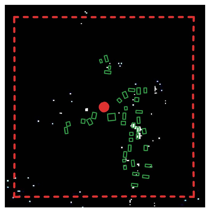
Clustering Events Spatially and Temporally
FIRMS fire detections can be dense and noisy, as the constellation consists of multiple satellites (NOAA-20 & NOAA-21) carrying the VIIRS instrument. With each satellite having a revisit time of 12 hours, and their orbits only being offset by 50 minutes, mid-latitudes experience 3-4 looks per day. Therefore it is very likely that the same event will be represented by multiple detections. To avoid overwhelming investigators with redundant validations, we group nearby detections into "events" using spatial and temporal clustering.
The clustering logic groups fire detections:
- Within the same geographic area (e.g. a buffered urban zone)
- That occur within a few days of each other
First, we calculate the date gaps to previous detections:
Then, these are used to cluster temporally, while the area_include_id is used to cluster spatially. So the combination of area_include_id and event_no is the key to our clusters:
Once clustered, we calculate the centroid of each event using:
Finally, we build the resulting model:
We also compute additional metadata for each event:
- Date range (start and end of detection)
- Distance between detections in the cluster
- Aggregated burn scar evidence and building damage
This clustering greatly reduces manual workload investigators now review one summarised event instead of dozens of nearly identical fire points.
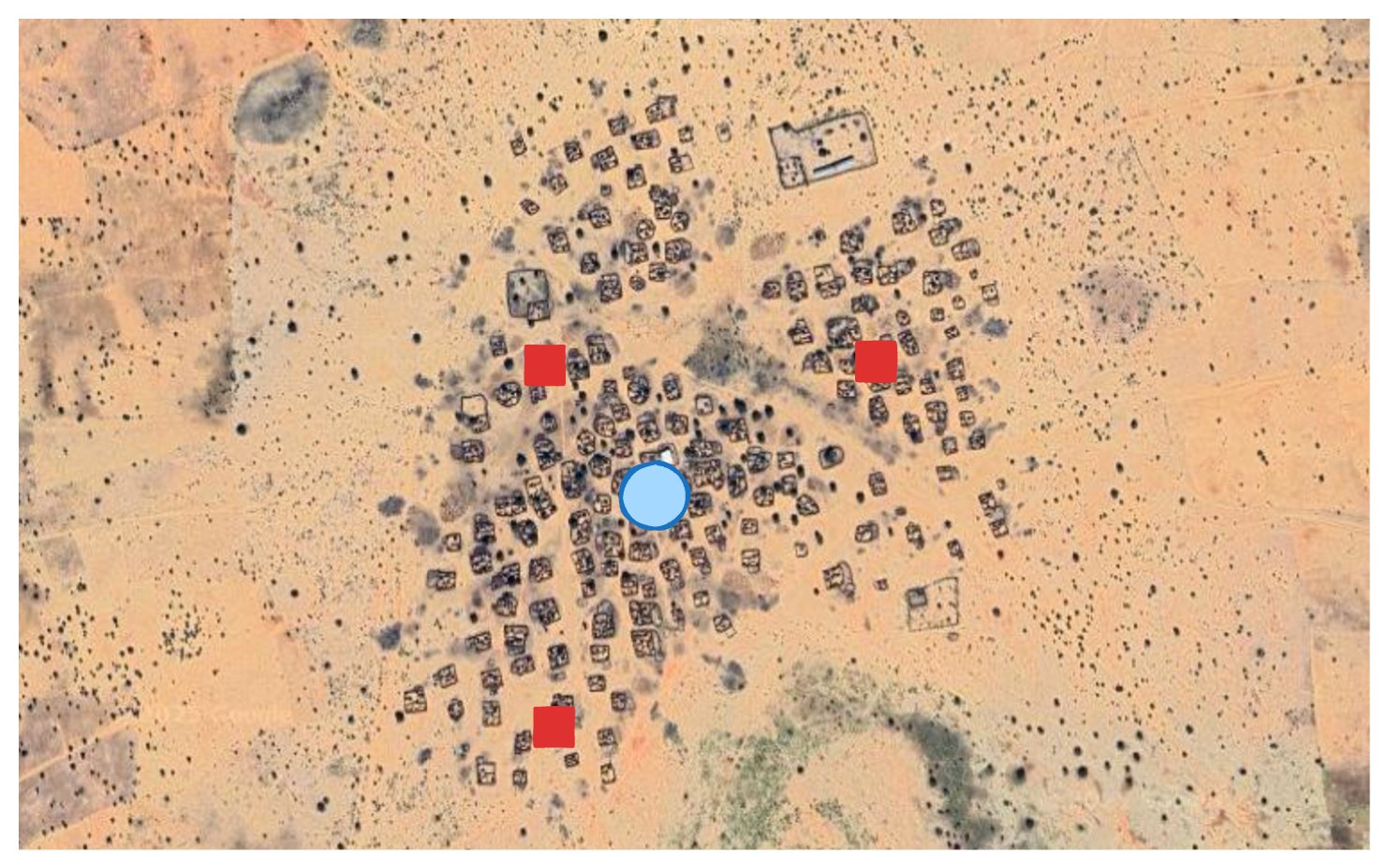
An example of a cluster of detections and their centroid. The red squares are FIRMS detections, the blue circle represents the centroid of this cluster.
Gaps, DAGs, and Targeted Retries
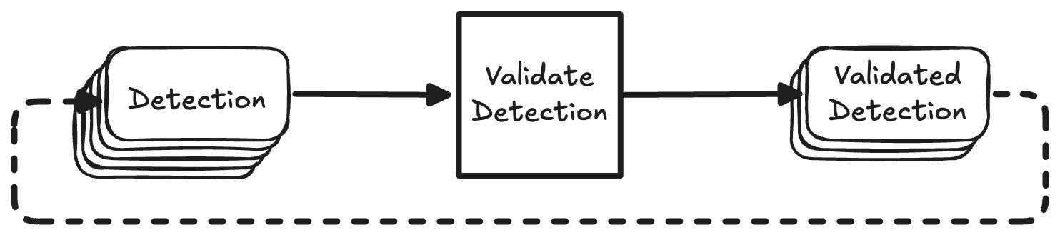
Sentinel-2 has a 5-day revisit cycle, and cloud cover is common. As a result, imagery is often unavailable in the days immediately after a fire detection. This introduces some non-deterministic behaviour: Some validations succeed immediately, others fail due to missing or unusable data.
Here lies the challenge: In a DAG, you can’t just query the output table to see which rows failed and retry them later, as that would create a cycle. DAGs must be acyclic and deterministic, and this retry logic breaks those rules.
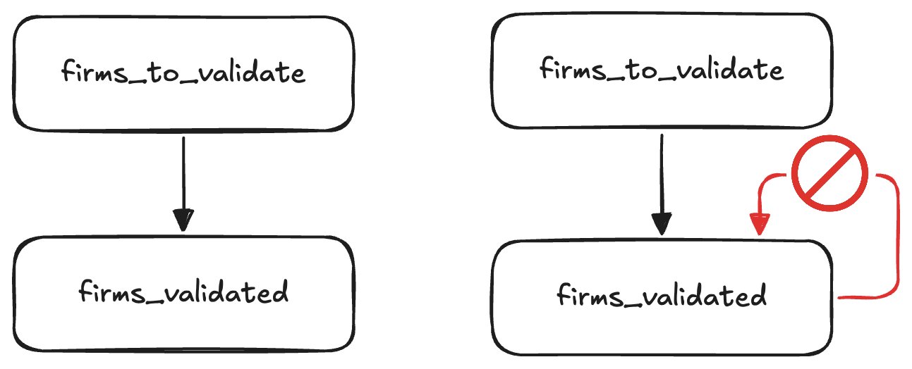
On the left we see the "ideal" scenario, where all validations succeed on the first try. On the right we'd check the output table to see which detections have already been validated successfully, using those to filter our input table. As you can see this turns our DAG into a directed graph, violating the assumption SQLMesh makes that a model can not depend on itself, directly or indirectly.
We have a few options to solve this problem:
- Only try once and accept the trade-off between latency (we can wait and only process after a few weeks) and failed validations.
- Simply re-process everything from the last period on every run.
- Maintain some external state in a table that is not managed by SQLMesh.
- Do a fixed number of retries at predefined delays.
Option 1 is the simplest solution, but we'd prefer to have at least some of the results sooner so investigators can start verifying and cross-referencing detections. This decreases the chances of evidence already having been removed from social media platforms by the time we do the verification. Option 2 is not really an option due to the validation being so expensive computationally, and at some point cost wise too. Option 3 felt like a hack, since one of the reasons to use SQLMesh for this project is that it can manage all tables and their states. By introducing external state, unnecessary complexity is introduced.
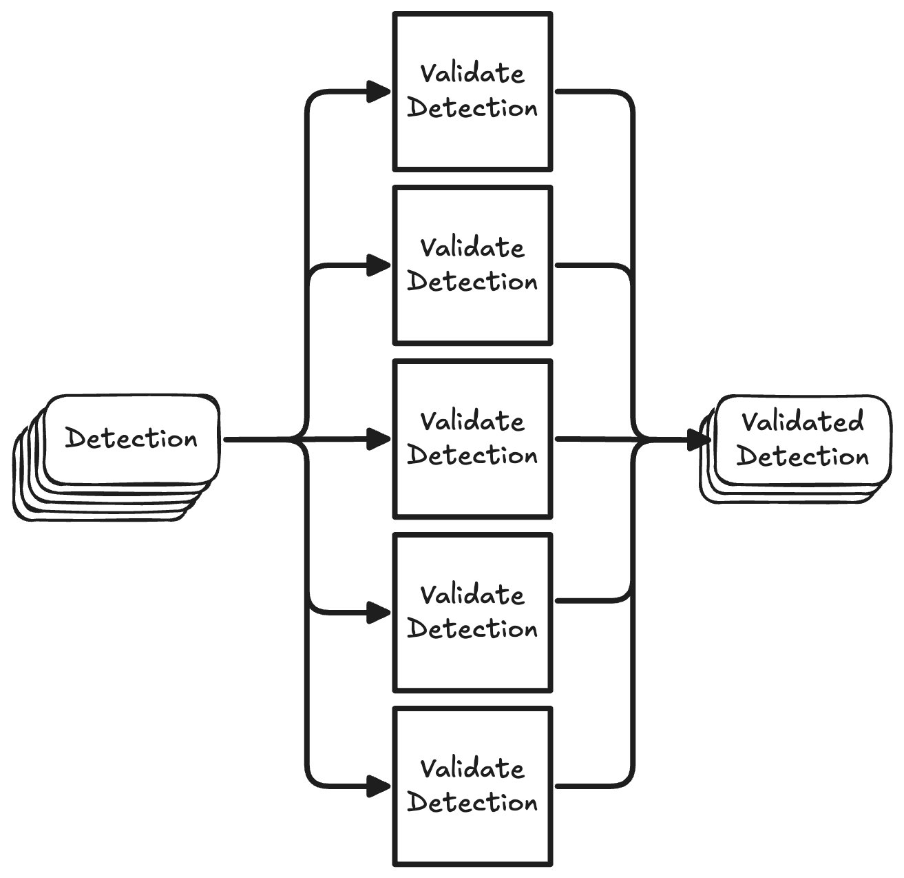
That leaves us with option 4. Luckily SQLMesh has two very useful features to accomplish this without copying and pasting a model a couple of times: Blueprints and macros. Blueprints let us define templates for models that will then be evaluated at parse time. Macros (in the broader computer science context) let us define reusable patterns that will be expanded to some desired code (SQL in our case).
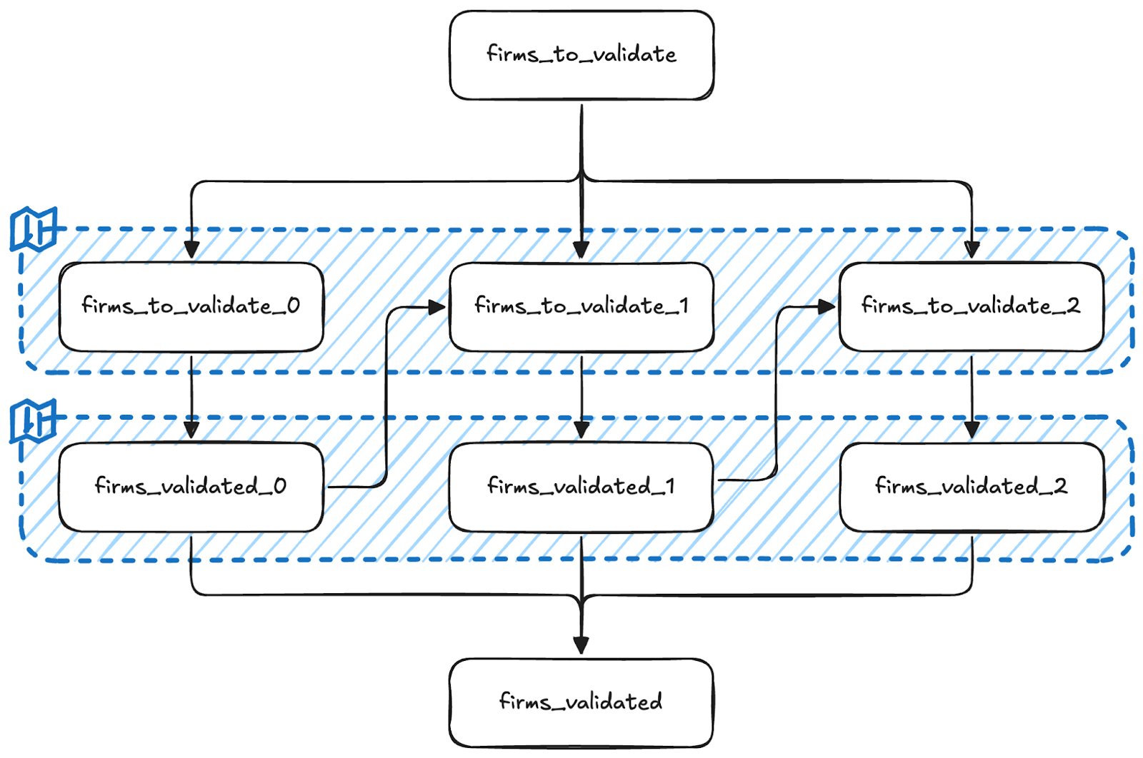
The combination of blueprints and macros lets us easily create multiple models for validation attempts at specific delays. The input for a blueprint is an array of mappings, where each mapping corresponds to a model that will be created physically by SQLMesh. In our case we have a try and day key in these mappings. Each retry checks the output from the previous run to exclude already validated detections. This allows us to selectively reprocess only the failed validations, without violating DAG structure or duplicating work.
This is the blueprint model we use to construct the input tables for our validation tries. This blueprint expands to 3 SQLMesh models:
intermediate.firms_to_validate_0,
intermediate.firms_to_validate_1 and
intermediate.firms_to_validate_2. The
firms_validated_0, firms_validated_1 and
firms_validated_2 models are created in a similar fashion. The diagram below shows the resulting models and their dependencies on each other.
As you can tell from the MODEL definition, we try at most 3 times at specific delays of 11, 16 and 21 days. These were chosen to have at least 2 passes of Sentinel-2 when we first try to validate a detection, but could of course be configured differently to decrease latency.
This model uses some SQLMesh macros to dynamically construct parts of the query.
- @variable_name:
@variable_nameor@{variable_name}if used inside model names. Access the user defined variable with the namevariable_name, can be defined globally, on a gateway level, in a blueprint or locally. We use it here to access blueprint variables. - @DEF:
@DEF([variable name],[expression])or@DEF([function name], [input, ...] -> [expression])Allows us to define a macro variable or function locally. In our case we use this to dynamically determine the upstream model that this model depends on. - @EVAL:
@EVAL([expression])Evaluates its arguments with SQLGlot's SQL executor. We use this to evaluate the expression@try_ - 1to look at the previous try. - @AND:
@AND([condition, ...])Combines a sequence of operands using theANDoperator, filtering out any NULL expressions. We use it here to combine the two conditions in theWHEREclause, since the second condition in the@IFmacro may beNULLand will be omitted in that case.
@IF: @IF([logical condition], [value if TRUE], [value if FALSE]) Allows components of a SQL query to change based on the result of a logical condition. We use it here to conditionally render the dependency on the output of the previous try.
Also note that for this model we explicitly define a name. For the models we've seen earlier the name is inferred based on the filename and path. SQLMesh does this when adding the following setting in your config.yaml:
So for example, the model defined in models/intermediate/firms.sql will automatically be named intermediate.firms.
Finally, the firms_validated model combines these tables.
Wrapping Up
Documenting war crimes presents numerous challenges, particularly in remote areas lacking media coverage. Automating key parts of the OSINV workflow enables large-scale, evidence-driven documentation, even amidst conflict.
What we gained
Significant improvements have been made to enhance the efficiency and robustness of the system, primarily in terms of speed and reliability:
- Validation is orders of magnitude faster: Previously taking hours, validation now completes in minutes.
- Zero manual intervention: After initial setup, the entire workflow up to human verification is fully automated, eliminating any manual steps.
- Incremental and consistent detections: The pipeline maintains an incremental dataset, ensuring previously processed data remains unchanged.
- Easy backfilling: SQLMesh allows effortless retroactive processing of new detections or imagery down to a specified start date. Although this slightly impacts consistency due to sequential numbering of clusters, it significantly improves flexibility.
This enables analysts to dedicate their time to complex tasks such as contextual analysis, cross-referencing, and verification, rather than manual data handling and duplicate removal.
Why this matters beyond Sudan
This pipeline is just the beginning. Designed to be open-source, modular, and adaptable, it can monitor burn events globally, from Ukraine to Myanmar with minor adjustments. For regions that have no or little natural fires, all that's needed is a config change.
Potential future enhancements include:
- Serverless compute deployment: Transitioning the pipeline to run on serverless compute, using object storage for databases, and publishing outputs as open datasets.
- Improved clustering methods: To enhance spatio-temporal clustering consistency, we are exploring better clustering techniques. While DBSCAN would be a good fit, it's not currently supported by DuckDB/spatial. An alternative is developing SQL-based transitive clustering focused solely on spatial proximity, simplifying the pipeline and reducing dependency on urban area filtering.
If you're involved in conflict documentation, geospatial tooling, or simply curious about the project, reach out to CIR or visit our Burnscar GitHub repository. Star the repo, open issues, or join discussions if you’d like to help.
Credits
Much credit for this project's success goes to the dedicated investigators at the Centre for Information Resilience’s Sudan Witness Project.
This project was made possible thanks to the foundational research and work of:
- Michael Cruickshank: https://github.com/MJCruickshank
- Mustafa A
- Tarig Ali: https://github.com/tariqabuobeida
- Mark Snoeck