Beyond Python: Internals, Performance, and Rust Integration (1/3)

Enrico Mosca

This post is the first in a three-part series. It explores how to overcome Python’s performance and maintainability challenges by understanding its internals and integrating it with Rust. As the old Yiddish saying goes (“Mann Tracht, Un Gott Lacht”), the agenda for this series may change, but ideally I would like to cover the following:
- Part 1 (this post):
We introduce the problem, discuss the impact of technical debt, and explore how Python works internally. - Part 2:
We’ll dive into how Rust works internally and why it’s an attractive choice for building high-performance, reliable components. - Part 3:
We’ll show how to bridge Python and Rust using PyO3, demonstrating practical ways to combine the strengths of both languages.
Introduction
Over the past decade, Python has surged to become one of the world’s most popular programming languages. Its simple yet powerful syntax has lowered the barrier to entry, enabling thousands of people, including those without traditional software engineering backgrounds, to write code and build applications. This accessibility has fueled Python’s growth across industries, from web development to data science. However, with this growth come challenges surrounding performance, maintainability, and scaling Python for complex applications.
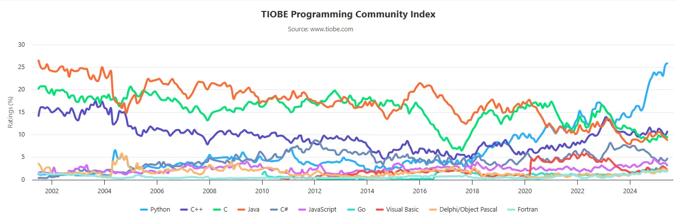
Python’s Popularity and Its Pitfalls
The rapid adoption of Python came with trade-offs. As organizations rushed to deliver new features and scale their systems — often leveraging the flexibility of cloud computing — many Python codebases grew organically. Unfortunately they often paid little attention to structure, documentation, or performance. The result? A proliferation of messy, hard-to-maintain code that can be slow and difficult to refactor.
If you’ve ever inherited a large Python project, you might recognize the symptoms:
- Little or no documentation
- Sparse (or absent) type hints
- Performance bottlenecks that are hard to diagnose
- Production issues cropping up on your first day
For years, the ease of scaling in the cloud made it tempting to ignore these problems. But as cloud costs rise and systems mature, the technical debt accumulated during this period is coming due.
The Cost of Technical Debt
Technical debt is more than just a metaphor. It has real, tangible costs. Slow code leads to higher infrastructure bills and frustrated users. Poorly structured projects make onboarding new developers a challenge. And a lack of type safety or documentation increases the risk of bugs and outages.
Today, many teams are realizing that the quick wins of the past have led to long-term headaches. There’s a growing desire for solutions that combine Python’s ease of use with greater reliability and performance.
Why Understanding Python Internals Matters
To address these challenges, it’s crucial to understand how Python works under the hood. By learning about Python’s execution model, memory management, and performance characteristics, developers can make informed decisions about optimization and refactoring. This knowledge also lays the groundwork for integrating Python with other languages such as Rust, that can help address its limitations.
Why Rust you ask? Well whether you like it or not is already part of this new paradigm with tools like uv, ruff, pydantic(v2) and polars.
Rust presents itself as a language that focuses on performace, reliability, and productivity. It even resembles Python in some ways.
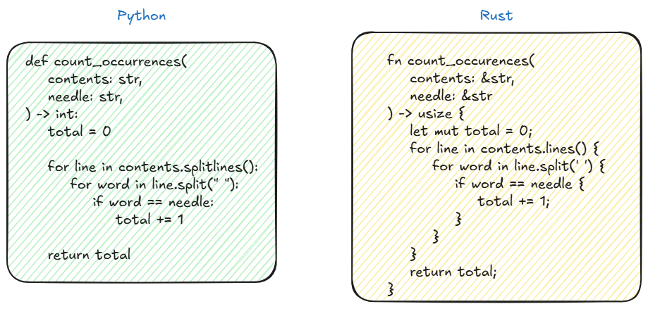
Similarities between Python and Rust.
How Python Works Internally?
The Python Execution Pipeline
Although you don’t need to know how Python works to have a successful career as a Python developer, it can be fun.
Let’s open our favorite terminal and type python to enter the Python’s interpreter in the so called interactive mode. Then we’ll just define a simple a function add that takes two arguments and returns their sum.
❯ python
Python 3.13.0b1 (main, Jun 25 2025, 10:34:23) [GCC 11.4.0] on linux
>>> def add(i1: int, i2:int)->int:
... return i1+i2
...
>>> add(1,3)
4
When we call the function with i1=1 and i2=3 we are successfully returning the result.
Cool, but how?
When a Python script is invoked, the interpreter initiates a sequence of transformations:
- Tokenize the source code Parser/lexer/ and Parser/tokenizer/.
- Parse the stream of tokens into an Abstract Syntax Tree (AST) Parser/parser.c.
- Transform AST into an instruction sequence Python/compile.c.
- Construct a Control Flow Graph (CFG) and apply optimizations to it Python/flowgraph.c.
- Emit bytecode based on the Control Flow Graph Python/assemble.c.
Let’s have a deeper look at each of these steps.
What the Tokenizer Does
The tokenizer (or lexical scanner) is the first step in processing Python source code. It reads the raw source code as a stream of characters and breaks it down into meaningful units called tokens. These tokens represent keywords, identifiers, operators, literals, punctuation, and even comments and whitespace where significant (such as indentation).
Each token is labeled with its type and includes metadata about where it appears in the source code (start and end line and column numbers). The tokenizer output is a sequence of these tokens, which is then passed to the parser for further processing.
What the Tokenizer Output Looks Like
When you use the built-in tokenize module, the output for a function like:
def add(i1: int, i2: int) -> int:
 return i1 + i2
would look like this
❯ python -m tokenize main.py
# name of the token, start position(line, char), end position
 ENCODING 'utf-8' start=(0, 0) end=(0, 0)
1: NAME 'def' start=(1, 0) end=(1, 3)
 NAME 'add' start=(1, 4) end=(1, 7)
 LPAR '(' start=(1, 7) end=(1, 8)
 NAME 'i1' start=(1, 8) end=(1, 10)
 COLON ':' start=(1, 10) end=(1, 11)
 NAME 'int' start=(1, 11) end=(1, 14)
 COMMA ',' start=(1, 14) end=(1, 15)
 NAME 'i2' start=(1, 16) end=(1, 18)
 COLON ':' start=(1, 18) end=(1, 19)
 NAME 'int' start=(1, 19) end=(1, 22)
 RPAR ')' start=(1, 22) end=(1, 23)
 RARROW '->' start=(1, 23) end=(1, 25)
 NAME 'int' start=(1, 25) end=(1, 28)
 COLON ':' start=(1, 28) end=(1, 29)
 NEWLINE '\n' start=(1, 29) end=(1, 30)
2: INDENT start=(2, 0) end=(2, 4)
 NAME 'return' start=(2, 4) end=(2, 10)
 NAME 'i1' start=(2, 11) end=(2, 13)
 PLUS '+' start=(2, 13) end=(2, 14)
 NAME 'i2' start=(2, 14) end=(2, 16)
 NEWLINE '\n' start=(2, 16) end=(2, 17)
3: DEDENT '' start=(3, 0) end=(3, 0)
 ENDMARKER '' start=(3, 0) end=(3, 0)
Each line represents a token, showing its position, type, and value.
Source code to AST
The stream of tokens produced by the tokenizer is then fed into a parser, which constructs the AST based on Python’s grammar. The AST is an high-level representation of the program structure without the necessity of containing the source code. Each grammar rule in the Python parser creates AST nodes as it recognizes language constructs. As parsing proceeds, the parser allocates new nodes as needed, calling the appropriate AST node creation functions and connecting them according to the code’s structure. This process continues incrementally as the parser matches tokens and grammar rules. If the parser encounters input that does not match any rule, it raises a syntax error and parsing ends.
We can get an idea of what this looks like by using the ast python’s package.
❯ python -m ast main.py
Module(
 body=[
 FunctionDef(
 name='add',
 args=arguments(
 posonlyargs=[],
 args=[
 arg(
 arg='i1',
 annotation=Name(id='int', ctx=Load())),
 arg(
 arg='i2',
 annotation=Name(id='int', ctx=Load()))],
 kwonlyargs=[],
 kw_defaults=[],
 defaults=[]),
 body=[
 Return(
 value=BinOp(
 left=Name(id='i1', ctx=Load()),
 op=Add(),
 right=Name(id='i2', ctx=Load())))],
 decorator_list=[],
 returns=Name(id='int', ctx=Load()))],
 type_ignores=[])
AST to CFG to bytecode to PyCodeObject
After the AST is generated, it undergoes some more simplification to reduce the numbers of nodes and subtrees. Next the CFG (control flow graph) is created; the CFG is a directed graph that models the flow of a program using basic blocks that contain intermediate representation of the code and that have a single entry point and possibly multiple exit points.
Using python-ta we can get an idea of what the CFG for your program looks like.
pip install python-ta
python
>>> import python_ta.cfg as cfg
>>> cfg.generate_cfg("main.py")
This generates a main.svg file in your folder which represents a basic block. It’s nothing more than some code that starts at the entry point and runs to an exit point.
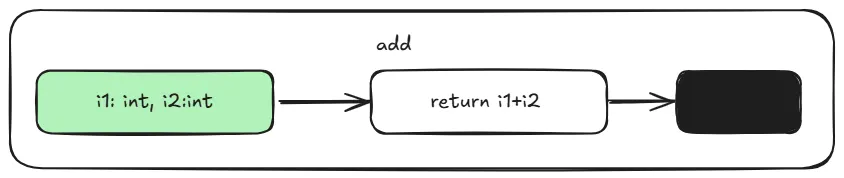
CFG representation of main.py
The Control Flow Graph (CFG) is further optimized (as implemented in Python/flowgraph.c). After these optimizations, pseudo-bytecode is produced. This pseudo-bytecode is an abstract, non-executable representation in which jump instructions refer to logical labels rather than concrete positions. When generating the final bytecode, these logical jumps are converted into actual instruction offsets, making the code executable by the Python Virtual Machine (PVM). A virtual machine is an emulated machine implemented in software, designed to support instructions similar to those of an actual hardware machine.
During this process, variable scopes are determined, the CFG is flattened into a linear sequence, pseudo-instructions are converted into real bytecode instructions, and jumps between blocks are resolved.
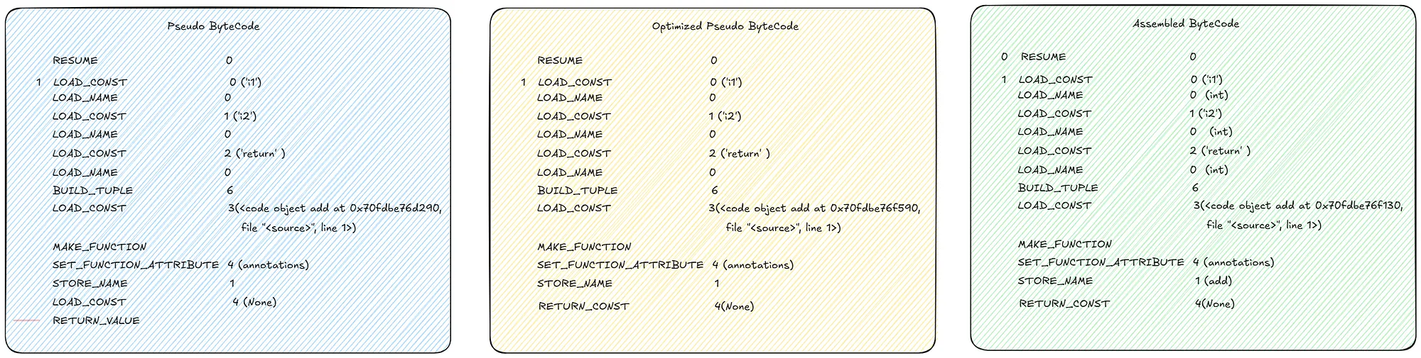
Comparison between different stages of bytecode, generated with https://github.com/iritkatriel/codoscope
In the example above there aren’t many differences since the code is quite simple.
Bytecode and PyCodeObject Structure
Once we have generated the sequence of bytecode instructions (opcodes), these are combined with essential metadata to create a PyCodeObject. This object is a fundamental part of CPython’s internals, it encapsulates compiled Python code and includes:
- Bytecode instructions: The opcodes that the Python Virtual Machine executes.
- Constants table: Literal values used within the code.
- Names table: Identifiers for variables and functions referenced by the code.
- Variable information: Details about local and global variables.
- Additional metadata: Such as line number tables, stack size requirements, and more.
The structure of PyCodeObject is defined in CPython’s source (see Include/code.h), with much of the compilation logic implemented in Python/flowgraph.c and it looks like this:
typedef struct {
 PyObject_HEAD
 int co_argcount;
 int co_nlocals;
 int co_stacksize;
 int co_flags;
 PyObject *co_code; // Bytecode
 PyObject *co_consts; // Constants
 PyObject *co_names; // Names
 PyObject *co_varnames; // Local variable names
 // ... more fields ...
} PyCodeObject;
If you are not familiar with C struct, you can easily think of this as a Python dataclass which would look
@dataclass
class PyCodeObject:
 co_argcount: int
 co_nlocals: int
 co_stacksize: int
 co_flags: int
 co_code: Any # Typically bytes or a custom object
 co_consts: Any # Typically tuple or list
 co_names: Any # Typically tuple or list
 co_varnames: Any # Typically tuple or list
 # ... more fields ...
Think of the PyCodeObject as a portable, intermediate representation of your Python code. The Python Virtual Machine interprets these instructions at runtime.
You may have seen a __pycache__ folder containing .pyc files. These are serialized PyCodeObjects, allowing Python to skip recompilation for faster startup.
When Python code is compiled, it produces a PyCodeObject, which the Python Virtual Machine (PVM) then executes.
You can inspect a PyCodeObject in Python using the dmodule:
>>> import dis
>>> from main import add
code = add.__code__
print(code.co_argcount) # 2 number of positional arguments
print(code.co_varnames) # ('i1', 'i2') a tuple containing the names of the
 # local variables
print(code.co_flags) # 3 number of flags for the interpreter
print(code.co_code) # b'\x95\x00X\x01-\x00\x00\x00$\x00' \
# string representing the sequence of bytecode instructions.
If we call list() on the byte string, then each byte returns it’s integer value and then we can get the huma readable name for the operation using dis.opname . This gets illustrated in the next snippet.
human_readable_co_code = list(code.co_code)
print(human_readable_co_code) # [149, 0, 88, 1, 45, 0, 0, 0, 36, 0]
>>> dis.opname[88]
'LOAD_FAST_LOAD_FAST'
>>> dis.opname[36]
'RETURN_VALUE'
Finally we can just call dis.dis to display the disassembly of the function. The number on the left represents the line number.
# The dis module supports the analysis of CPython bytecode by disassembling it
>>> dis.dis(code)
 1 RESUME 0
 2 LOAD_FAST_LOAD_FAST 1 (i1, i2)
 BINARY_OP 0 (+)
 RETURN_VALUE
In the next section, we’ll explore how the Python Interpreter and Virtual Machine work together to execute your code.
Bytecode to Execution
We finally have something simple enough to run at runtime. This is when the PVM (Python Virtual Machine) comes into play. PVM has a stack based design (as opposed to a registry based) so the bytecodes is executed within stack-based frames using a large switch statement (in C implementations). This replaces opcodes with actual machine code.
while (1) {
 // Fetch the next bytecode instruction.
 int opcode = NEXTOP();

 switch (opcode) {
 case LOAD_CONST: {
 // Load a constant onto the stack.
 PyObject *const_value = GET_CONST();
 STACK_PUSH(const_value);
 break;
 }
 case BINARY_ADD: {
 // Pop two values, add them, and push the result.
 PyObject *right = STACK_POP();
 PyObject *left = STACK_POP();
 PyObject *result = PyNumber_Add(left, right);
 STACK_PUSH(result);
 break;
 }
 // Handle other opcodes...
 default:
 // Unknown opcode error handling.
 PyErr_SetString(PyExc_SystemError, "unknown opcode");
 return NULL;
 }
}
Each function called pushes a new entry (i.e. a frame) onto the call stack. When a function returns, its frame is popped off the stack.
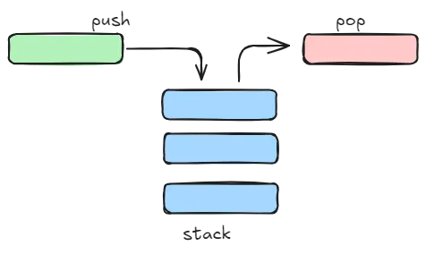
High level representation of a fifo queue.
A frame is a collection of information and context related to a chunk of code corresponding to each function call, and it is destroyed on-the-fly.
Let’s describe what happens under the hood with our simple function.
Please note that for this example we are going to use Python 3.10 since Python 3.13 introduces some optimization that makes the process less clear.
Let’s invoke dis.dis on our simple add function
Python 3.10.15 (main, Apr 16 2025, 10:06:53) [GCC 11.4.0] on linux
Type "help", "copyright", "credits" or "license" for more information.
>>> import dis
>>> from main import add
>>> dis.dis(add)
 2 0 LOAD_FAST 0 (i1)
 2 LOAD_FAST 1 (i2)
 4 BINARY_ADD
 6 RETURN_VALUE
>>> add(i1=5,i2=3)
8
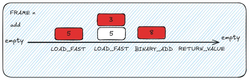
High level representation of how stack works.
Assuming that we want invoke add(i1=5, i2=3) :
- The PVM creates a new stack frame with an empty evaluation stack and local variables are mapped (i1 and i2 are assigned their slots)
- The PVM’s main loop reads the first bytecode (0: LOAD_FAST 0)
- This triggers the corresponding case in the giant switch statement.
- The value 5 is pushed into the stack (the stack has now 1 value). - The PVM’s main loop reads the next bytecode pointer (2: LOAD_FAST 1)
- This triggers the corresponding case in the giant switch statement.
- The value 3 is pushed into the stack (the stack has now 2 values). - The PVM’s main loop reads the next bytecode pointer (4: BINARY_ADD)
- The function pops the 2 values from the stack and pushes the result
- The value 8 is pushed into the stack (the stack has now 1value). - The PVM’s main loop reads the next bytecode pointer (6: RETURN_VALUE)
- Pops the value from the top of the evaluation stack
- Tears down the current frame
- Returns control to the calling frame (passing the value)
And this is how a simple python code function that adds two number together is internally!
Practical Example: Diagnosing a Performance Bottleneck with Internals Knowledge
Knowing how the internal works can be useful to identify and explain bottlenecks when doing code reviews. Let’s compare two implementations of a function that takes as an input a list of integers and returns the squared sum of it’s elements. In the slow version we are accessing the elements in the array by index.
# Slow function
def sum_of_squares_slow(nums:list)->int:
 total = 0
 for i in range(len(nums)):
 total += nums[i] ** 2 # access the array by index
 return total
In the fast version of the code we use an iterator.
# Faster version
def sum_of_squares_fast(nums:list)->int:
 total = 0
 for num in nums: # Uses efficient iterator protocol
 total += num ** 2
 return total
If we use timeit to compare the executes time we’ll see that the second function is on average ~ 15% faster.
import statistics
import timeit
>>> print(statistics.mean(timeit.repeat(lambda: \
sum_of_squares_slow(list(range(1000))), repeat=10,number=100000))
4.704 # seconds
>>> print(statistics.mean(timeit.repeat(lambda: \
sum_of_squares_fast(list(range(1000))), repeat=10,number=100000))
4.0667 # seconds
To understand why this happens, we can use dis.dis(sum_of_squares_slow) and dis.dis(sum_of_squares_fast) to see what the bytecode looks like.
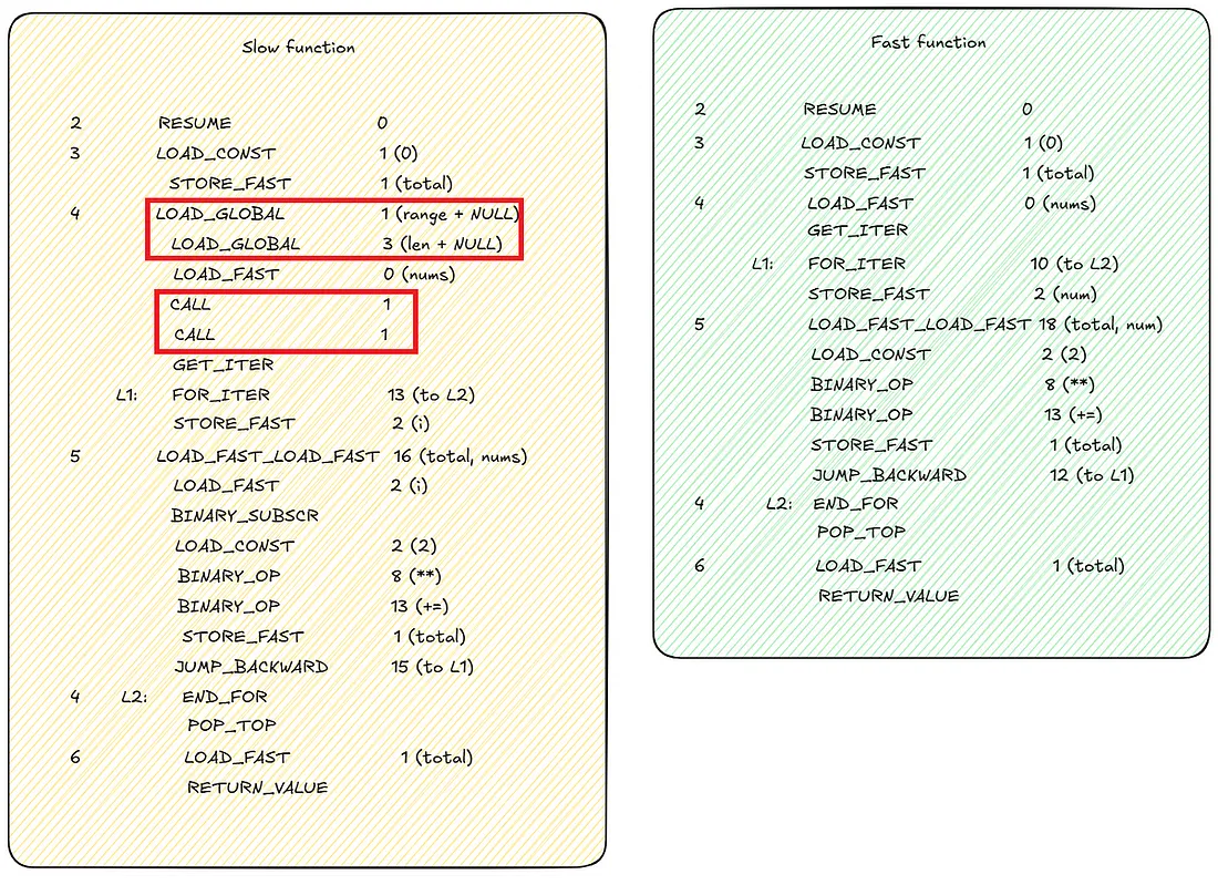
Bytecode comparison between slow and fast sum_of_square function.
We immediately notice that the fast function has a more compact set of instructions. Accessing the array by index require extra calls to load range and len functions in memory, as well extra CALL to actually call them.
Recap
In this post, we explored why Python’s popularity has led to new challenges, and took a detailed look at how Python works under the hood. Python’s internal libraries were introduced and used to explain how the source code is transformed into bytecode. Python’s virtual machine FIFO memory management and the CPython runtime were briefly discussed. Finally we looked at how to use Python’s internals knowledge to understand bottlenecks in our code.
What’s Next
In the next article, we’ll dive into Rust’s internals and see why it’s such a powerful companion to Python for performance-critical tasks.